
The Physical Setup
In 1999 the Numerical Relativity Group at AEI performed the first numerical simulation of a grazing collision of two non-rotating black holes with unequal masses (gr-qc/0012079). This physical setup required a full 3D modeling. Until that time only situations could be performed if they were symmetric in a special way – e.g. axially symmetric such as a precise head-on collision – such that they could be reduced to a 2D Simulation – which was computationally much easier.
The simulation was performed on a newly inaugurated supercomputer at the National Center for Supercomputing Applications where the Numrel Group had exclusive access before its public opening. The computations lasted three weeks and produced several dozens of gigabytes of data, an amount that was challenging to handle at that time.
The Apparent Horizons
Black holes are characterized by their event horizon, which is defined as the region from which nothing can ever escape into infinity. This concept is difficult to model numerically because the notion of “ever” and “infinity” requires knowledge of the entire future and space, which with finite numbers and technically limited computational power is beyond its capabilities. Only in the far future one can say that somewhere in the past there was an event horizon at a given time step.
Fortunately, there is the property of an “apparent horizon” that can be used as an alternative concept as its definition depends merely on local properties of the spacetime. Together with a theorem that every apparent horizon must be surrounded by an event horizon, the concept of an “apparent horizon” gives a numerically graspable clue of black holes. Eventually the result of the merger process will be a single, rotating black hole.
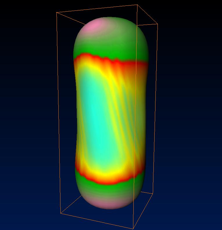
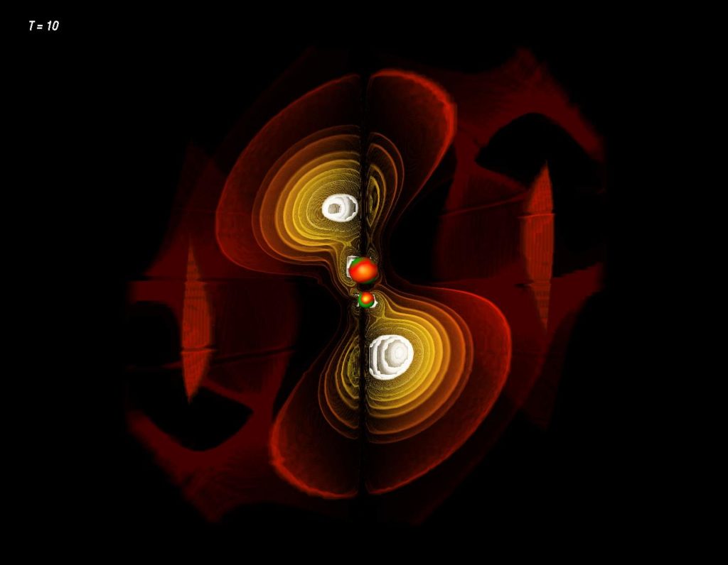
Apparent Horizons can “jump” and “pop up”. At a certain instant of time, a common apparent horizon is formed, initially looking like a peanut-shape. The colorization indicates the curvature of the horizon: What looks like a sphere here (i.e., in the coordinates chosen for this simulation), is not a sphere in reality, but some oddly shaped blob. Yellow indicates zero curvature (flat!), red is positive, but smaller than one (weakly spherical), green is larger than one (strong spherical curvature). In some regions the curvature is even negative (i.e. concave, beyond yellow).
The regions of negative curvature are quite prominent at horizon creation – the cyan/transparent areas of the surface around the xy equatorial plane, surrounded by the yellow regions of zero surface curvature. The curvature corresponds well to the visual coordinate appearance of the apparent horizon, as these equatorial areas are saddle-like.
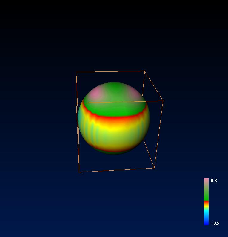
The Movie shows the Apparent Horizons of the two initial Black Holes, which are essentially two spheres, whereby the colors indicate the gaussian curvature along the surfaces. Gaussian curvature of a surface is equal to 1/r2, where r is the local radius of curvature at the surface point. Of course, in general relativity the local radius has to be measured using metric distances, not coordinate distances. The movie shows the coordinate appearance of the Apparent Horizon, but the metric gaussian curvature. The gaussian curvature is normalized here to the area of the surface, such that a sphere would appear red independently of its size. Yellow stands for flat areas, blue to negative curvature (hyperbolic curvature, saddle-like surfaces) while green and finally rose represent highly positivly curved surface areas.
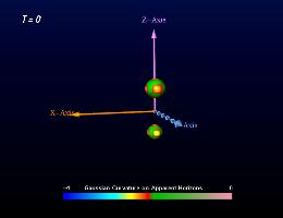
Due to its local definition, the Apparent Horizon is not a causal structure. Therefore it may jump into existence at specific times. This is the case with the colliding black holes, too. At T=10.36 the common Apparent Horizon of the two black holes jumps into existence (in truth, the Apparent Horizon was not computed at each evolution time step, so it might already have existed somewhat longer, but at least it is for sure that there was none at the beginning).
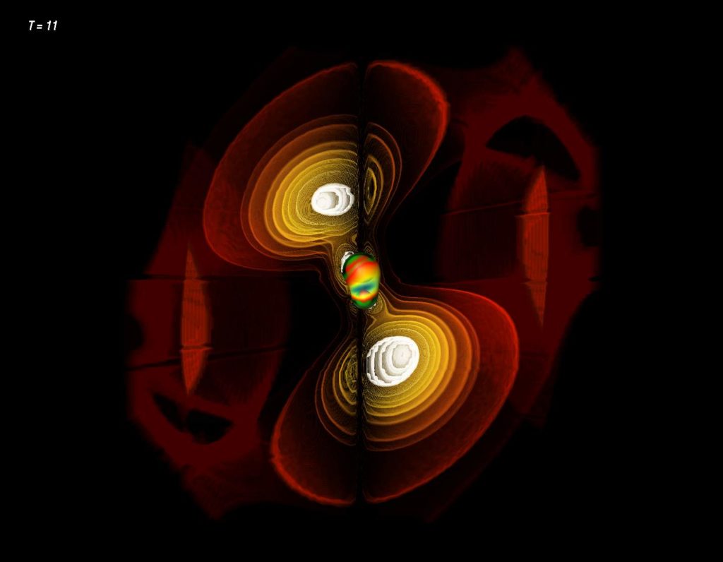
At first, the enveloping outer Apparent Horizon has some negative curvature at the equator areas. General Relativity predicts that any black hole must become a Schwarzschild or, in the case of rotation, a Kerr Black Hole (no-hair-theorem). So any perturbation of another kind of black hole must be radiated away and the distorted black hole must become a Kerr Black Hole after sufficient time. So does this newly generated black hole. The outer Apparent Horizon become more spherical (better: elliptic, to approach the Kerr-Black Hole appearance) during the evolution.
Through the transparently rendered surface of the Apparent Horizon one may still see the two inner parts of the Apparent Horizon, corresponding to the two initial black holes. The upper one tends to move forward into x-direction, indicating its linear momentum. Due to this linear momentum the newly created black hole which originates from this black hole merger, has an angular momentum around the y-axis (it becomes a Kerr Black Hole). When concentrating on the gaussian curvature structures along the outer apparent horizon surface, one can follow this kind of rotation of the structures in counter-clockwise rotation around the y-axis.
Evolution of the apparent horizons during the grazing collision. During formation the common apparent horizon just “pops into existence” (which happens at T=10.36M in this simulation), indicating that both black holes are contained in a common event horizon that resides even further out. The common horizon appears to grow because the coordinates used for this simulation are “falling into” the black hole, while in reality the final horizon will be of constant size.
Soon after creation the outer apparent horizon tends toward becoming elliptical, approaching the shape of a Kerr Black Holes event horizon. The curvature structures again show the rotation of the features aorund the y axis, corresponding to the angular momentum of the final rotating Kerr Black Hole.
The Gravitational Field
The gravitational field is described by various quantities indicating different properties. They can be understood as the “stretch” and “compression” in the multiple directions in space and time. For depiction of the structural evolution of a black hole merge, the Newman-Penrose pseudo-scalars are suitable quantities as they have certain intuitive interpretations. There are five such complex quantities denoted Ψ0, Ψ1, Ψ2, Ψ3 , Ψ4. This means there are ten independent numbers at each point in space and time. Hereby Ψ4 is the most interesting one of them as it corresponds to the outgoing gravitational energy.
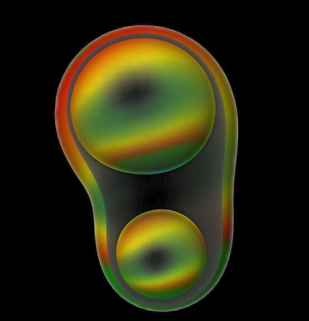
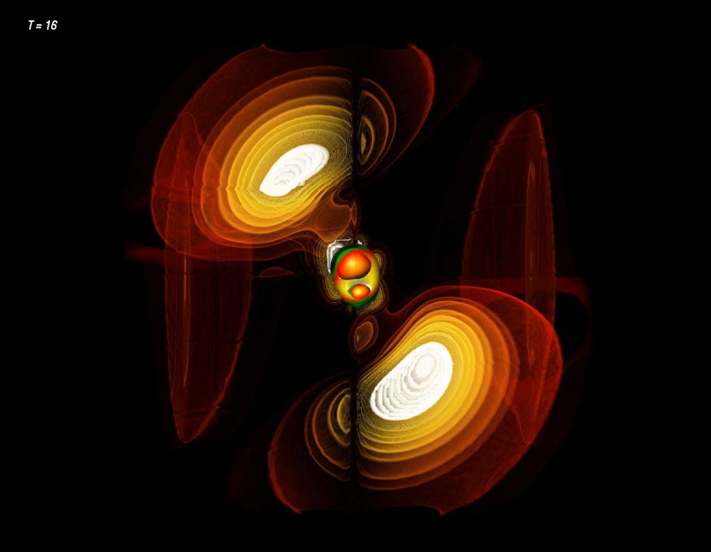
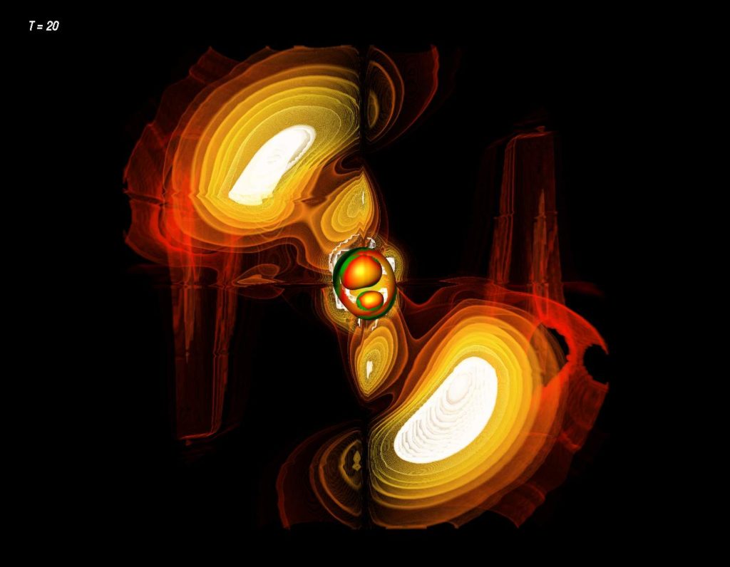
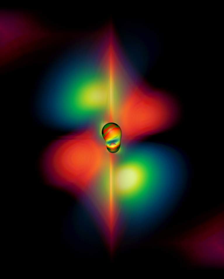
The Positive Part of Re Ψ4
Ψ4 is a complex quantity consisting out of two numbers. For an astrophysical situation as simulated here the imaginary part is zero in the plane of motion of the two initial black holes. Thus only the real part is of primary interest for this scenario when focusing on the plane of motion. Even further reducing the amount of data, the regions of spacetime where the real part of Ψ4 is positive depicts a clear structure of two “bubbles” emerging from the two black holes.
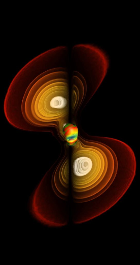
This image depicts various levels of intensity in the Ψ4 field as thin transparent surfaces, nested like the skins of an onion. This highest intensity level is rendered white, while the lowest intensity level (some small value larger than zero) is rendered dark red
In this simulation, the common apparent horizon forms at T=10.36M, where M is a mass unit. A time unit of 1M can be understood as the time that light takes to travel a distance – in flat space – that corresponds to the Schwarzschild radius of a mass M.
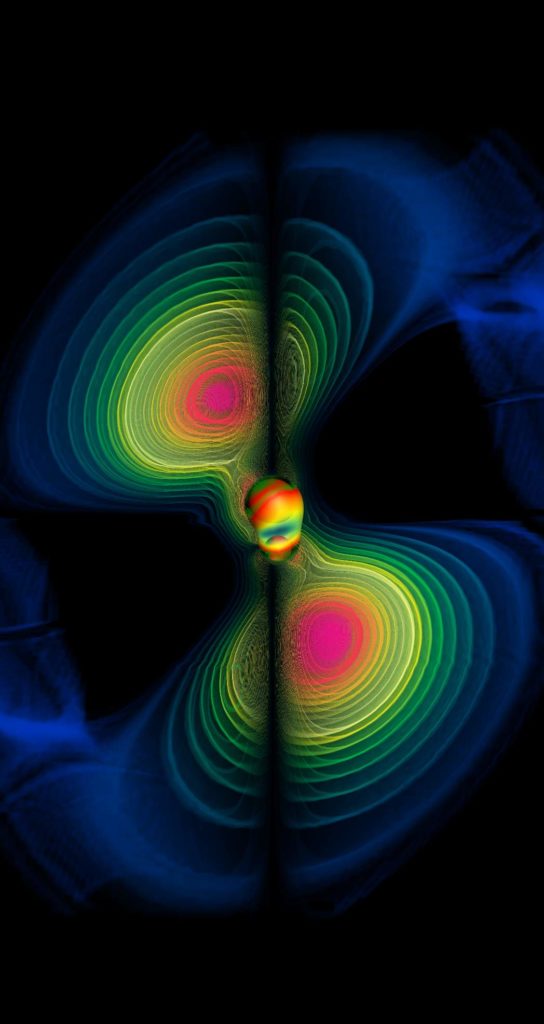
Alternative version of the color-coding to utilize all colors for the data field.
The Full Signature of Re Ψ4
The Newman-Penrose field Re Ψ4 – which indicates the gravitational wave’s polarization – shown with positive parts in blue-green, negative regions in red. The lobe-like structure from the former images shows up blue-green here. The negative regions fill out the remaining space; thus it is sufficient to show the positive part only (as in the former section) to get a basic understanding of spatial distribution.

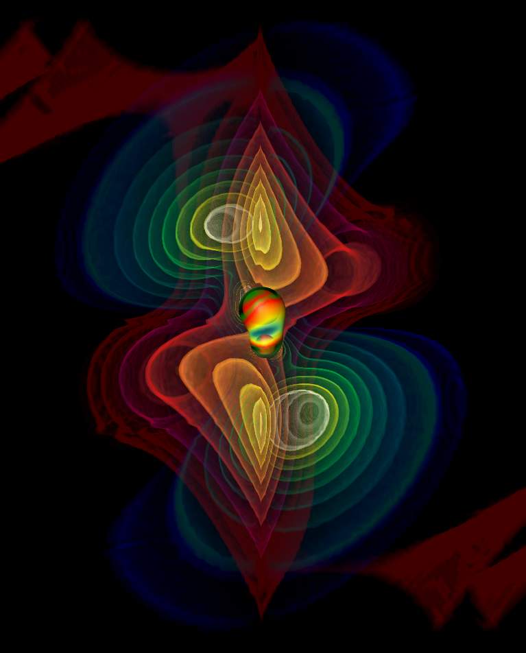
Using the technique of “onion colormaps” (or “volumetric isolevels”) the structural differences of the field become more prominent. While the positive part (blue) is like two emerging blobs, the negative part (red) looks more “heart-shaped” at this moment in time.
When depicting the evolution of the full-signature Re{Ψ4} field (red: positive, blue: negative), a rotational structure becomes evident in the resulting outburst. Thus, from the initial status of two non-rotating black holes on a grazing trajectory a rotational pattern is produced.
The Imaginary Part of Ψ4
As mentioned above, the imaginary part of Im{Ψ4} is all zero in the plane of motion (the zx-plane in the coordinate system used here) for the scenario discussed here. Nevertheless outside this exact plane the field exhibits interesting features: Negative areas are rendered as blue volumetric isolevels, positive areas as red/violett volumetric isolevels. During evolution, blue pulses (negative valued wave fronts) emerge and are followed by red (positive) pulses, and vice versa. For a specific point in space, e.g. some point along the y-axis, this alternating of signs in Im{Ψ4} corresponds to the well-known wave forms of an oscillation.

×-polarization component of the outgoing gravitational energy, as indicated by Im{Ψ4}.
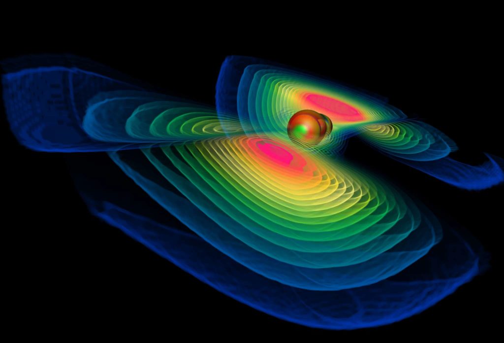
The Full Complex Structure of Ψ4
The Ψ4 Weyl Scalar is a complex quantity, which can be interpreted under some assumptions as the `outgoing gravitational’ wave. The real part indicates the even parity component, the imaginary part stands for the odd part. For axisymmetric cases, the odd part, and therefore Im{Ψ4} is zero.
For full 3D structures, this is no longer the case. Re{Ψ4} is rendered as red volumetric isolevels, as in the former video, but seen from a different view position. Additionally, Im{Ψ4}2 is shown as blue volumetric isolevels.
While Re{Ψ4} shows two `pulses’ running towards the (+x,0,+z) “up” and (-x,0,-z) “down” direction and becomes quite chaotic, even unstructured, at later time steps, Im{Ψ4} appears as two pulses running in opposite directions towards (0,+y,0) “right” and (0,-y,0) “left”. It seems to be mainly moving orthogonal to the Re{Ψ4} pulse direction. The geometric structure of Im{Ψ4} remains remarkably clean at later time steps, it does not show the chaotic behavior of Re{Ψ4}.
Re{Ψ4}² in red, Im{Ψ4}² in blue.
Video Compilation: Grazing Black Holes, 1999
Putting all of the above together, the following video was compiled from various animation sequences based on the 1999 data set.
The video of the BH Collision data depicts various sequences of the properties as discussed above.